1.算法流程
DDPM的算法流程如下:
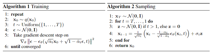
训练阶段重复以下步骤:
- 从数据集中采样$x_0$
- 随机选取 time step $t$
- 生成高斯噪声 $\epsilon \in \mathcal N(0,I)$
- 调用模型预估 $\epsilon_{\theta}(\sqrt{\bar{\alpha _t}}x_0+\sqrt{(1-\bar{\alpha_t})}\epsilon_t,t)$
- 计算噪声之间的 MSE loss: $\parallel \epsilon_t-\epsilon_{\theta}(\sqrt{\bar \alpha_t}x_0+\sqrt{(1-\bar\alpha_t)}\epsilon_t,t)\parallel^2$
逆向阶段采样如下步骤进行采样:
- 从高斯分布采样$x_T$
- 按照 $T,…,1$ 的顺序进行迭代:
- 如果 $t=1$,令$z=0$; 如果 $t>1$, 从高斯分布中采样 $z\sim \mathcal{N}(0,I)$
- 学习出均值 $\mu_\theta(x_t,t)=\frac{1}{\sqrt{\alpha_t}}(x_t-\frac{1-\alpha_t}{\sqrt{1-\bar\alpha_t}}\epsilon_\theta(x_t,t))$, 学习方差 $\sigma_t=\sqrt{\frac{1-\bar\alpha_{t-1}}{1-\bar\alpha_t}\cdot\beta_t}$ , 即 $\sqrt{\tilde{\beta}_t}$
- 通过重参数技巧采样 $x_{t-1}=\mu_\theta(x_t,t)+\sigma_tz$
- 经过以上过程的迭代,最终恢复 $x_0$ .
2.源码分析
DDPM 文章以及代码的相关信息如下:
- Denoising Diffusion Probabilistic Models 论文
- 本文分析的Pytorch源码:https://github.com/tqch/ddpm-torch
训练阶段
以cifar10数据集为例,在 train.py 中进行前向传播计算Loss:
 1def train(self, evaluator=None, chkpt_path=None, image_dir=None):
 2        #无关代码已省略
 3        #......
 4        global_steps = 0
 5        for e in range(self.start_epoch, self.epochs):
 6            self.stats.reset()
 7            self.model.train()
 8            results = dict()
 9            if isinstance(self.sampler, DistributedSampler):
10                self.sampler.set_epoch(e)
11            with tqdm(self.trainloader, desc=f"{e + 1}/{self.epochs} epochs", disable=not self.is_leader) as t:
12                for i, x in enumerate(t):
13                    if isinstance(x, (list, tuple)):
14                        x = x[0]  # unconditional model -> discard labels
15                    global_steps += 1
16                    self.step(x.to(self.device), global_steps=global_steps)
17                    t.set_postfix(self.current_stats)
18                    results.update(self.current_stats)
19                    if self.dry_run and not global_steps % self.num_accum:
20                        break
21           #.....
- 第16行调用
step()方法:
 1def step(self, x, global_steps=1):
 2    loss = self.loss(x).mean()
 3    loss.div(self.num_accum).backward()  # average over accumulated mini-batches
 4    if global_steps % self.num_accum == 0:
 5        nn.utils.clip_grad_norm_(self.model.parameters(), max_norm=self.grad_norm)
 6        self.optimizer.step()
 7        self.optimizer.zero_grad(set_to_none=True)
 8        # adjust learning rate every step (e.g. warming up)
 9        self.scheduler.step()
10        if self.use_ema and hasattr(self.ema, "update"):
11            self.ema.update()
12    loss = loss.detach()
13    if self.distributed:
14        dist.reduce(loss, dst=0, op=dist.ReduceOp.SUM)  # synchronize losses
15        loss.div_(self.world_size)
16    self.stats.update(x.shape[0], loss=loss.item() * x.shape[0])
- 第2行调用
loss()方法,train_losses 定义在GaussianDiffusion中, 计算噪声间的 MSE Loss.
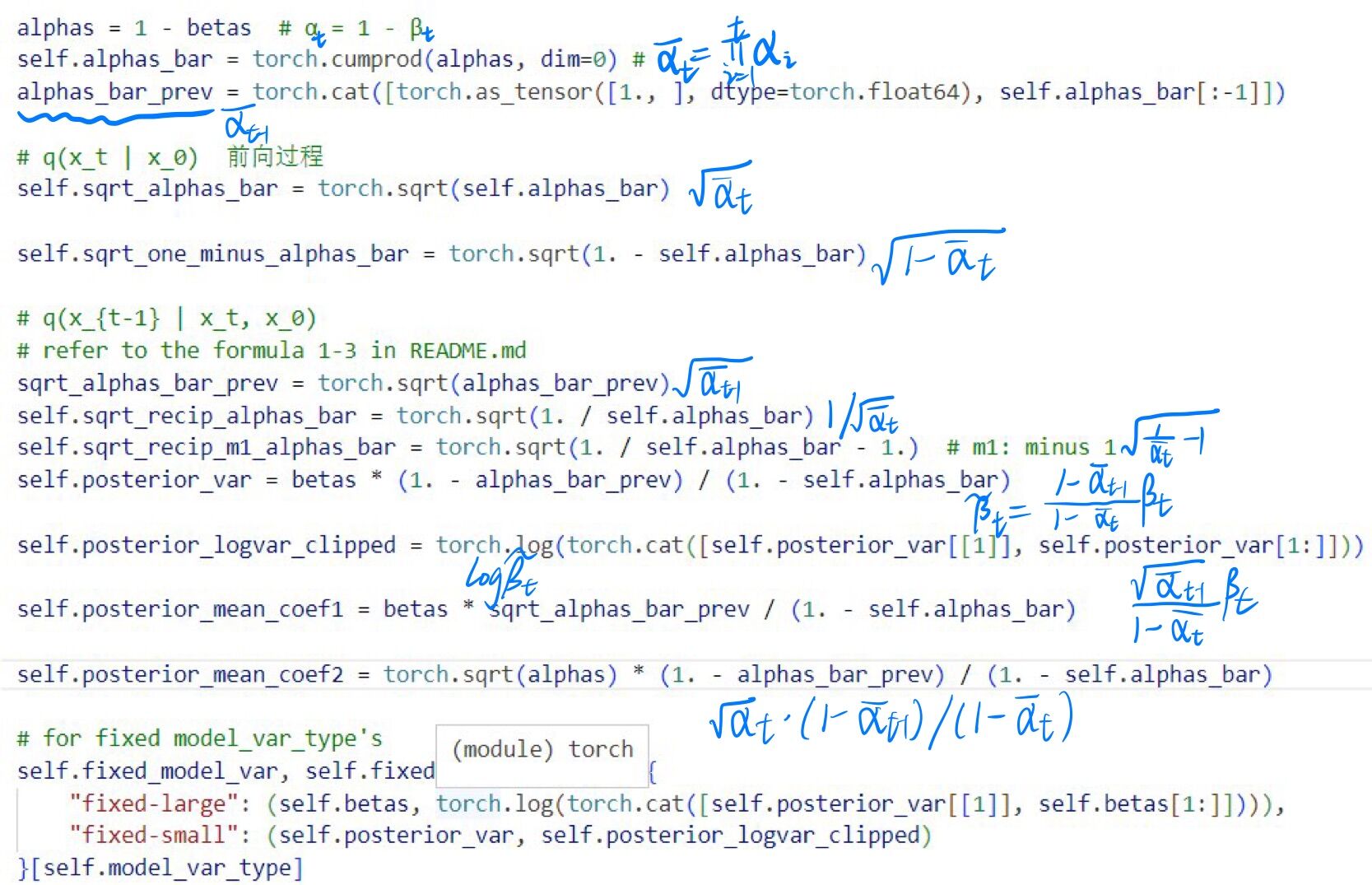
进入 GaussianDiffusion 中, 看到初始化函数中定义了诸多变量, 在注释中使用公式的方式进行说明:
下面进入train_losses函数中:
 1def train_losses(self, denoise_fn, x_0, t, noise=None):
 2    # 添加噪声
 3    if noise is None:
 4        noise = torch.randn_like(x_0)
 5    x_t = self.q_sample(x_0, t, noise=noise)
 6    # calculate the loss
 7    if self.loss_type == "kl":     # kl: weighted
 8        #......
 9    elif self.loss_type == "mse":  # mse: unweighted
10        assert self.model_var_type != "learned"
11        if self.model_mean_type == "mean":
12            target = self.q_posterior_mean_var(x_0=x_0, x_t=x_t, t=t)[0]
13        elif self.model_mean_type == "x_0":
14            target = x_0
15        elif self.model_mean_type == "eps": # 默认为esp
16            target = noise
17        else:
18            raise NotImplementedError(self.model_mean_type)
19        model_out = denoise_fn(x_t, t)
20        losses = flat_mean((target - model_out).pow(2))
21    else:
22        raise NotImplementedError(self.loss_type)
23    return losses
- 第15行:
self.model_mean_type默认为eps,模型学习的是噪声,因此target即为第3行定义的noise,即 $\epsilon_t$ - 第5行:调用
self.q_sample计算 $x_t$, 即公式 $x_t=\sqrt{\bar{\alpha _t}}x_0+\sqrt{(1-\bar{\alpha_t}}\epsilon_t$ - 第19行:
denoise_fn是定义在unet.py中的Unet模型,该模型的输入和输出大小相同,结合第5行得到的 $x_t$,模型预估出的噪声为 $\epsilon_{\theta}(\sqrt{\bar{\alpha _t}}x_0+\sqrt{(1-\bar{\alpha_t})}\epsilon_t,t)$ - 第20行:计算两个噪声之间的MSE:$\parallel \epsilon_t-\epsilon_{\theta}(\sqrt{\bar \alpha_t}x_0+\sqrt{(1-\bar\alpha_t)}\epsilon_t,t)\parallel^2$,并利用反向传播算法训练模型
上面第5行调用的self.q_sample定义如下:
 1@staticmethod
 2    def _extract(
 3            arr, t, x,
 4            dtype=torch.float32, device=torch.device("cpu"), ndim=4):
 5        if x is not None:
 6            dtype = x.dtype
 7            device = x.device
 8            ndim = x.ndim
 9        out = torch.as_tensor(arr, dtype=dtype, device=device).gather(0, t)
10        return out.reshape((-1, ) + (1, ) * (ndim - 1))
11
12def q_sample(self, x_0, t, noise=None):
13        if noise is None:
14            noise = torch.randn_like(x_0)
15        coef1 = self._extract(self.sqrt_alphas_bar, t, x_0)
16        coef2 = self._extract(self.sqrt_one_minus_alphas_bar, t, x_0)
17        return coef1 * x_0 + coef2 * noise
- 第15行中
self.sqrt_alphas_bar是 $\sqrt{\bar\alpha_t}$ - 第16行中
self.sqrt_one_minus_alphas_bar是 $\sqrt{1-\bar\alpha_t}$ - 第17行,即计算 $x_t=\sqrt{\bar\alpha_t}x_0+\sqrt{1-\bar\alpha_t}\epsilon_t$
- 第 2 行的
_extract在代码中经常被使用到, 看到它只需知道它是用来提取系数的即可. 引入输入是一个 Batch, 里面的每个样本都会随机采样一个 time step t, 因此需要使用gather来将 $\bar{\alpha_t}$之类选出来, 然后将系数 reshape 为 [B, 1, 1, ….] 的形式, 目的是为了利用 broadcasting 机制和 $x_t$ 这个Tensor 相乘.
广播(Broadcasting)机制: 是 numpy 对不同形状(shape)的数组进行数值计算的一种方式。
前向的训练阶段代码较为简单, 下面分析逆向阶段。
逆向阶段
逆向阶段代码定义在GaussianDiffusion 中: